
Introduction - why predicting short-term volatility matters When markets move fast, anticipating...
Introduction: Understanding Short-Term Drivers of Gold
Gold is often seen as both a safe haven and a mirror of global economic sentiment.
In the short term, its price doesn’t move because of slow structural forces like mining output or long-term demand, but rather because of rapid shifts in markets and expectations.
Daily or weekly price changes usually reflect how investors react to new information about currencies, interest rates, inflation, and financial risk.
To capture these short-term movements, we can build a data-driven model that links gold’s daily returns to economic and financial indicators that move on a similar timescale.
- When the US dollar strengthens, gold often falls because it becomes more expensive for investors who hold other currencies.
- When interest rates or bond yields rise, holding gold becomes less attractive since it doesn’t pay interest.
- On the other hand, if inflation increases or investors expect higher prices in the future, gold tends to gain value because it’s viewed as a hedge against inflation.
- Periods of financial stress or market volatility also tend to push investors toward gold as a safe haven.
- Finally, changes in energy prices, such as oil, can influence inflation expectations and therefore indirectly affect gold.
The following article explores how neural networks, specifically Long Short-Term Memory (LSTM) models, can forecast short-term gold price movements by learning complex, time-dependent relationships between macroeconomic drivers such as the US dollar, market volatility, and energy prices.
Feature Engineering and Model Design
To capture short-term price movements effectively, the model must rely on features that reflect daily or weekly market dynamics rather than slow structural changes.
For this reason, we include both gold’s own lagged returns and external variables such as changes in the US dollar index, market volatility (VIX), oil prices, and major equity indices.
Together, these inputs describe how investors’ risk perception, inflation expectations, and currency valuations shift from one day to the next.
Before feeding them into the model, the data are normalised and aligned so that each feature represents the same observation window, ensuring the network learns consistent temporal patterns.
Among the different machine-learning options, Long Short-Term Memory (LSTM) networks are well suited for this task because they can recognise sequences and dependencies over time.
Unlike a standard feed-forward neural network that treats each observation as independent, an LSTM keeps track of recent context through its internal memory cells, allowing it to model how today’s gold return depends on signals from the last few days.
Compared with tree-based models such as XGBoost or Random Forest, which often perform well on tabular data, the LSTM can directly capture temporal ordering and lag interactions without manually engineering time-shifted features.
It is also more flexible than econometric approaches like ARIMA, which assume linear relationships and fixed lag structures.
Forecasting Strategies and Model Variants
There are several ways to structure the forecasting process depending on the desired time horizon.
A. Direct multi-step approach
In the direct multi-step approach, one LSTM model predicts several future days at once: For example, the next five trading days (5 days vector). Its output layer contains five neurons, allowing the network to learn how short-term price movements unfold jointly.
B. Recursive approach
The recursive approach predicts one day ahead, then feeds each forecast back into the model to predict the following day.
This setup is simple and fits naturally with daily updates, but forecast errors can accumulate as the horizon extends.
C. Mixed horizon approach
The mixed-horizon setup uses separate models for different timescales such as a one-day model for short-term trading signals, five-day model for intermediate momentum patterns, and a 21-day model for broader trend detection. In this approach, each horizon is modelled by its own network with separate weights and a single scalar output dedicated to that specific forecast period.
Strictly speaking, in Options A and B, the LSTM produces a continuous forecasted time series,
whereas in Option C, the model generates separate point forecasts for specific horizons that can later be combined into a broader, coarse-grained time profile.
Please note that all the models are trained on returns rather than absolute price levels, since returns are typically more stationary and easier for machine-learning algorithms to learn from. After forecasting the return sequences, these predictions are then translated back into price forecasts by compounding the predicted returns with the most recent observed price.
Model Performance and Forecast Interpretation
Across all configurations, the models capture gold’s overall direction, but their accuracy expectedly declines with the forecast horizon.
 Option A: The model captures the general price direction but reacts slowly to turning points and underestimates volatility, resulting in weak explanatory power (R² ≈ 0.08).
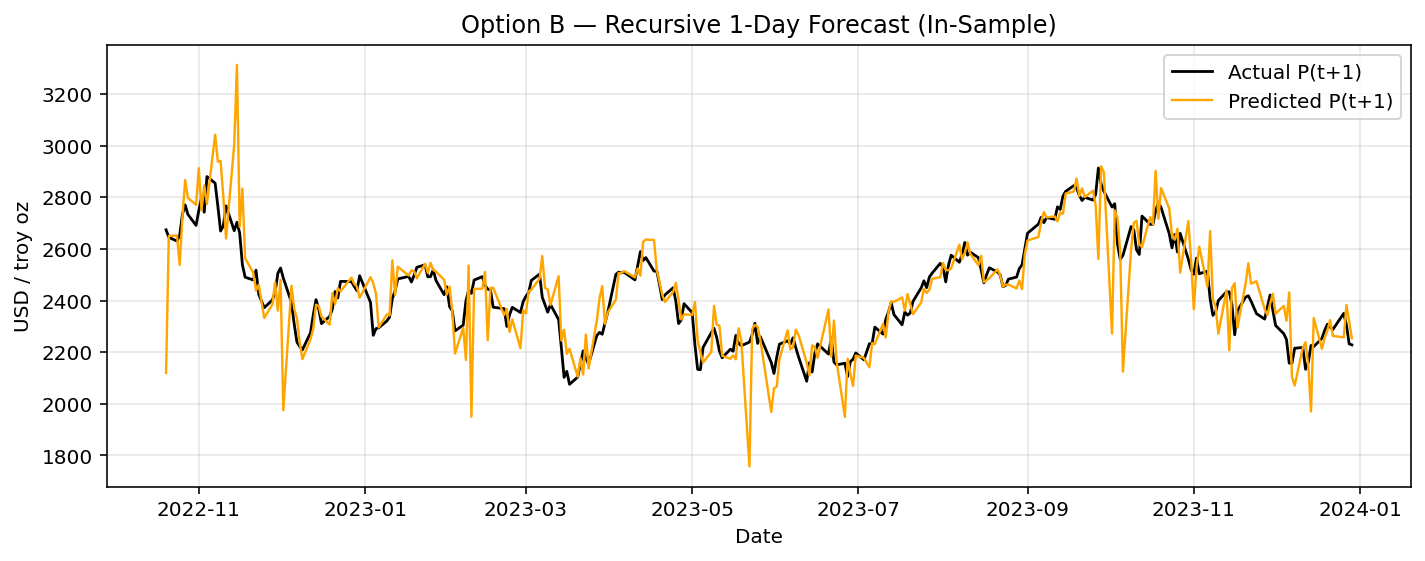
Option B: The recursive 1-day model follows overall trends well and maintains directionality over several days, though noise and small overshoots show minor error accumulation.
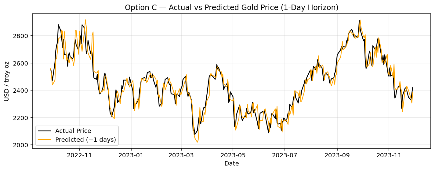
Option C (1 day): This specialised short-term model tracks daily movements almost perfectly, achieving the best fit and highest accuracy across all setups.
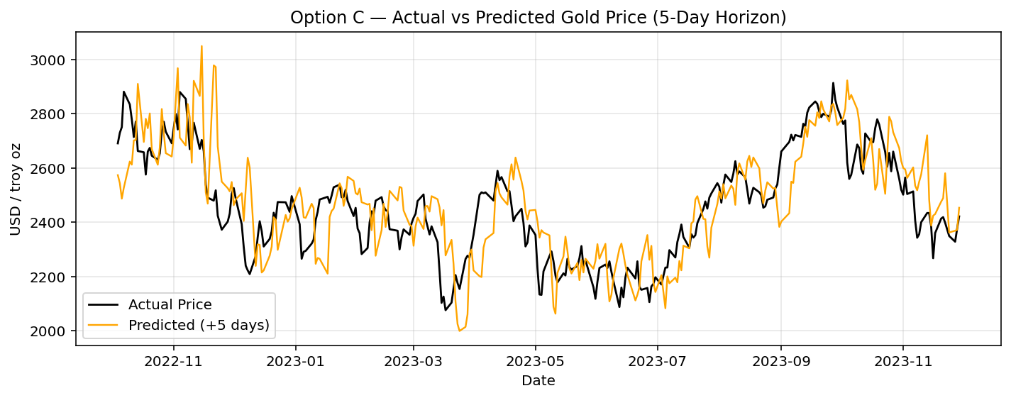
Option C (5 days): Predictions align closely with weekly swings while remaining smoother than actual prices, balancing responsiveness with stability.
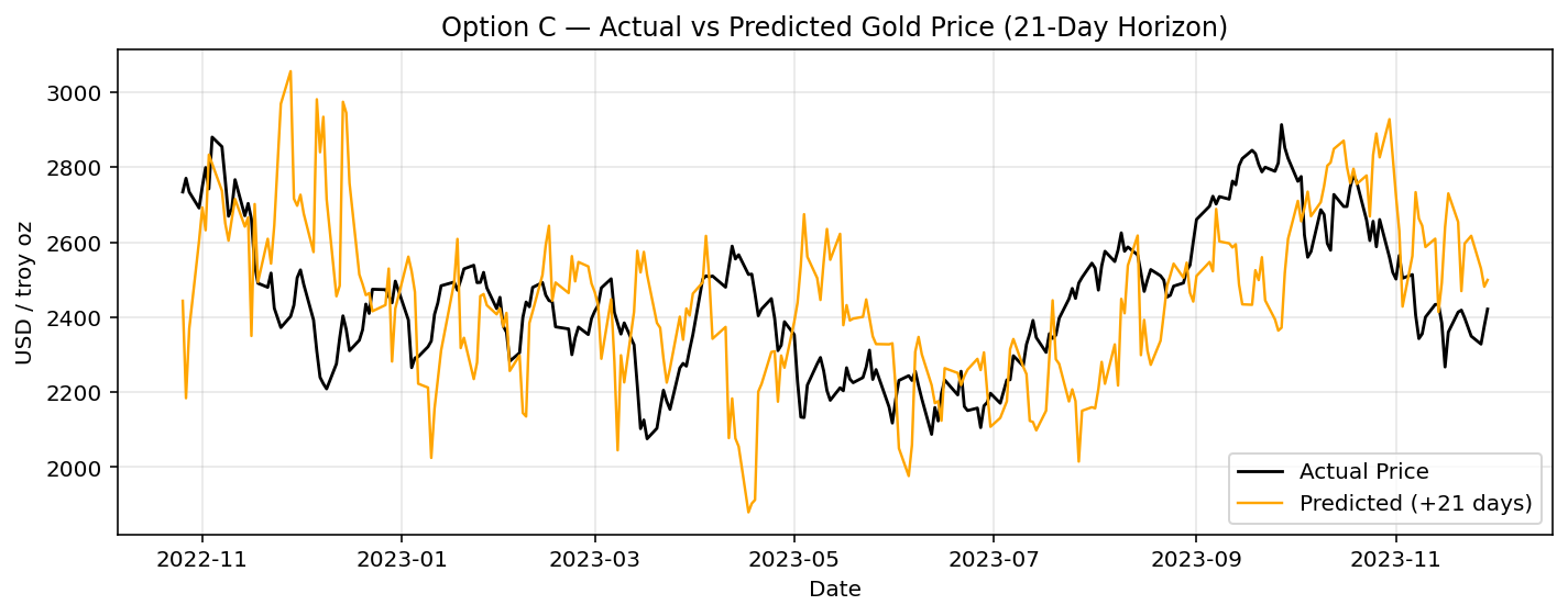
Option C (21 days): The long-horizon model captures broader market cycles but misses short-term fluctuations and turning points, reflecting its focus on trend detection rather than day-to-day moves.
Quantitative Comparison of Forecast Horizons
At short horizons of around one day, the models clearly capture a predictable structure. All approaches achieve errors of roughly 2–3 %, with coefficients of determination (R²) in the range of about 0.8 to 0.85. This indicates that short-term fluctuations in gold prices follow patterns that the models can reliably learn and reproduce.
Over a medium horizon of five days, the situation changes. The recursive model Option B performs best because it leverages the fine-grained daily micro-dynamics and carries them forward step by step. The direct multi-step approach Option A, by contrast, accumulates small inconsistencies across horizons, which compound into noticeable biases over several days. The separate-horizon model Option C treats five-day returns as independent targets and therefore captures a weaker, more aggregated signal with lower explanatory power.
At a long horizon of about 21 days, predictability largely collapses. Random fluctuations dominate the price movements, and any systematic signal fades into noise. As a result, the models lose explanatory strength, and the coefficient of determination even turns negative, showing that a simple mean forecast would outperform these long-term predictions.
| Option | Horizon | MAE (USD) | MAPE (%) | R² | Comment |
|---|---|---|---|---|---|
| A | 5 days | 146 | 6.0 | 0.08 | weak multi-step direct model |
| B | 5 days (recursive) | 78 | 3.2 | 0.58 | best medium-term performer |
| C | 1 day | 57 | 2.3 | 0.85 | top short-term accuracy |
| C | 5 days | 106 | 4.4 | 0.51 | decent but below recursive |
| C | 21 days | 183 | 7.5 | −0.51 | no predictive signal |
MAE (mean absolute error): The average absolute difference between predicted and actual prices. It shows the typical size of an error, measured in USD
MAPE (mean absolute percentage error): The average absolute error expressed as a percentage of the actual value. It shows the relative forecasting accuracy
R² (coefficient of determination): Measures how well the model explains the variance in the actual data. A value near 1.0 indicates excellent explanatory power; values near 0 mean the model is no better than predicting the mean; negative values mean it performs worse than that.
Conclusion: What We Learned from LSTM Forecasting
What did we actually gain by using an LSTM neural network to forecast gold prices, instead of relying on classical approaches such as ARIMA, linear regression, or simpler RNNs? In short, the LSTM allowed us to capture nonlinear, multi-factor, and state-dependent relationships that traditional models cannot represent. Gold price dynamics are influenced by complex, interacting drivers like USD strength (DXY), volatility sentiment (VIX), and oil or equity movements. These relationships are not constant over time: For example, gold’s sensitivity to DXY changes when market volatility spikes. Unlike ARIMA, which assumes linear and stationary behaviour with fixed lag dependencies, the LSTM learns these nonlinear conditional effects directly from the data, without manual feature engineering. It also remembers patterns of variable length thanks to its gated memory structure, allowing it to detect sequences such as “gold tends to mean-revert after three strong up days when DXY is rising,” something no static lag model could express.
Note: The gates in an LSTM determine how much of the current input, previous hidden state, and stored cell state are retained, updated, or passed forward, thereby controlling how past and present information contribute to the next prediction.
Another major advantage is the ability to handle multiple correlated inputs simultaneously. Whereas ARIMA is univariate by design (and VAR models require explicit specification of cross-dependencies), an LSTM can naturally integrate several time series and infer their joint impact on the target. This results in significantly higher short-term explanatory power: our 1-day LSTM achieved R² values around 0.83–0.85, compared to typical 0.2–0.4 for ARIMA on daily gold. In essence, we doubled the amount of variance explained at short horizons. However, the gain diminishes as the forecast horizon extends, because the further we project into the future, the weaker and less stable those short-term dependencies become. For the extended horizons, the limiting factor is not model capacity but the lack of predictable structure in the data itself.
As a next step, we could perform model tuning to optimise the LSTM’s architecture and training parameters, such as the number of units, dropout rate, learning rate schedule, or lookback window length to extract the maximum achievable signal from the available data. However, this should be done within the inherent limits of the data’s predictive structure, since no amount of tuning can recover information that simply isn’t present or stable in the time series.