Forecasting Volatility: How machine learning helps time risk in markets

Introduction - why predicting short-term volatility matters

When markets move fast, anticipating risk matters more than reacting to it. A 21-day forward volatility forecast offers a tactical edge across several domains from structured products to options and risk management.

Choosing the right model for volatility forecasting

When predicting volatility, GARCH models are often the first tool people reach for. They’re clean, statistical frameworks that model volatility as a function of past returns. But GARCH is purely univariate - that means it only sees the asset’s own return history - and it’s reactive, not proactive. If a large move happened yesterday, GARCH will assume higher volatility today. But it won’t know why that move happened, nor will it anticipate shocks from earnings, macro releases, or geopolitical risks. It’s a mechanistic, not causal model and in today’s information-rich markets, that can be limiting.

If you prefer models that are more feature-aware, and can learn patterns across multiple signals, tree-based models like XGBoost or Random Forests offer a powerful upgrade. You can feed them sentiment scores, macro surprises, volume anomalies, or VIX changes, and they’ll pick up nonlinear patterns - like “volatility rises when sentiment falls and bond yields spike.” Plus, with tools like SHAP values, you can interpret exactly which signals are driving a volatility spike.

When volatility depends on time-dependent structures such as price momentum, news impact, or earnings cycles, LSTMs and Transformer models shine. These deep learning models can pick up long-term dependencies, but come with the usual caveats: data hunger, risk of overfitting, and a tendency toward black-box behaviour unless carefully constrained.

Finally, if you believe markets operate under distinct volatility regimes like calm, volatile, or panic, then Hidden Markov Models (HMMs) offer an elegant solution. They can uncover regime switches based on latent state dynamics and even help you relate those shifts back to observable drivers like inflation surprises or monetary policy pivots.

No single model is perfect. The best choice depends on your goal: explainability, adaptability, anticipation or speed. In this blog, we use XGBoost, a supervised learning model that balances predictive accuracy with interpretability which makes it ideal for forecasting short-term volatility.

Designing features that capture market dynamics

For this analysis, we focus on Tesla (TSLA), a stock known for its high volatility, media exposure, and sensitivity to both company-specific news and broader market sentiment. These characteristics make it an ideal candidate for exploring how different signals can help predict short-term market turbulence.

To forecast volatility effectively, many start with the basics - namely returns. Just like traditional models such as GARCH, we begin by analysing Tesla’s daily return series. These returns contain valuable information about recent market shocks, trends, or quiet periods. By calculating lagged returns and rolling averages or standard deviations, we get a picture of how volatile Tesla has been over different horizons, such as 5, 10, or 21 days. These rolling metrics provide baseline estimates of recent volatility.

But price returns alone don’t tell the full story. We enhance our model with volume-based features, which add another layer of market insight. Trading volume reflects how many shares change hands on a given day. Spikes in volume can indicate investor reactions to news, increased uncertainty, or coordinated institutional activity. By including lagged and rolling statistics of Tesla’s trading volume, we capture these behavioural signals that often precede or coincide with market volatility.

Next, we expand the view to include broader market context, using the S&P 500 returns. Tesla’s volatility is rarely isolated from macro conditions. Large swings in the S&P 500 often ripple into high-beta stocks like Tesla. Lagged and rolling features of S&P 500 returns allow our model to account for systemic stress or rallies that might impact Tesla indirectly, such as during market-wide corrections or euphoric runs.

Finally, we introduce sentiment and forward-looking risk expectations through the VIX, often called the market’s “fear index.” The VIX measures the implied volatility of S&P 500 options. It reflects how volatile traders expect the market to be over the coming weeks. By including percentage changes in the VIX and its rolling patterns, we capture shifts in investor sentiment and perceived risk. These signals can help our model anticipate, rather than merely react to, upcoming periods of stress.

Altogether, by layering features from Tesla’s own behaviour, market-wide movements, trading activity, and forward-looking risk indicators, we build a much richer and more responsive volatility forecasting model than what traditional return-only models can offer.

1. return_ features

• Lags: lag_1, lag_3, lag_5, lag_10, lag_21, lag_42

• Rolling means: roll_mean_5, roll_mean_10, roll_mean_21, roll_mean_42

• Rolling stds: roll_std_5, roll_std_10, roll_std_21, roll_std_42

2. Volume_ features

• Lags: lag_1, lag_3, lag_5, lag_10, lag_21, lag_42

• Rolling means: roll_mean_5, roll_mean_10, roll_mean_21, roll_mean_42

• Rolling stds: roll_std_5, roll_std_10, roll_std_21, roll_std_42

3. sp500_return_ features

• Lags: lag_1, lag_3, lag_5, lag_10, lag_21, lag_42

• Rolling means: roll_mean_5, roll_mean_10, roll_mean_21, roll_mean_42

• Rolling stds: roll_std_5, roll_std_10, roll_std_21, roll_std_42

4. vix_change_ features

• Lags: lag_1, lag_3, lag_5, lag_10, lag_21, lag_42

• Rolling means: roll_mean_5, roll_mean_10, roll_mean_21, roll_mean_42

• Rolling stds: roll_std_5, roll_std_10, roll_std_21, roll_std_42

Note: The numerical suffix indicates the time horizon over which the return, change, or variability is measured, for example, over the past 5, 10, 21, or 42 days.

How well does the model predict volatility?

For this analysis, we focus on the period from January 2020 to December 2024, capturing a diverse market environment including the COVID-19 crash, recovery, inflation shocks, and monetary policy tightening cycles. Our target variable is the 21-day forward realised volatility of Tesla’s stock, calculated as the rolling standard deviation of daily returns over the next 21 trading days. This window approximates one trading month and aligns well with typical short-term risk horizons used by traders. To avoid lookahead bias, we only use information available up to the prediction date, and we train/test the model on chronologically ordered data. After engineering over 60 lagged and rolling features from returns, volume, market indices, and VIX, we split the dataset into an 80% training and 20% testing window, preserving the temporal structure. 

The below plot comparing predicted and true 21-day realised volatility for Tesla shows a strong alignment between the model’s forecasts and actual volatility outcomes over the 2020–2024 period. While short-term spikes (especially during crisis events) remain challenging to capture precisely, the model effectively tracks broader volatility trends, including major upswings and downswings. The blue dashed line (predicted volatility) tends to move in tandem with the black line (true volatility), suggesting that the XGBoost model trained on market returns, volume, and macro signals like VIX and S&P500 returns is well-calibrated to capture the underlying volatility dynamics. Some lag or smoothing of peak amplitudes is noticeable, which is typical for models designed to generalise well and avoid overfitting to short-term noise. Overall, this result indicates useful predictive power, especially for volatility timing decisions or structuring short-dated derivatives like weekly or monthly options.

Explaining model predictions with SHAP

To better understand how our model arrives at its volatility predictions, we use SHAP, a powerful tool for interpreting machine learning models. Following two visual outputs:

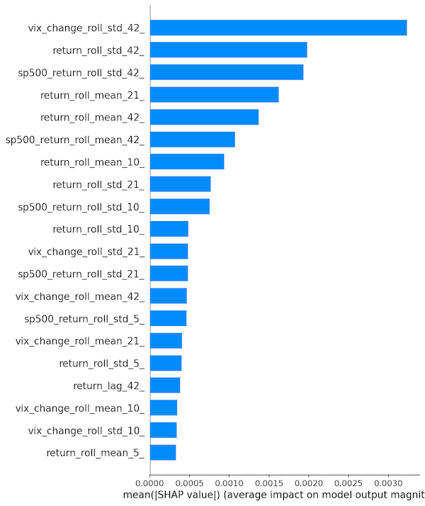
Observations:

• The model draws heavily from volatility patterns, especially longer-term volatility (42-day window) in both TSLA and the broader market. This reinforces that recent instability across the market has predictive value for Tesla’s short-term volatility.

Observations:

• High vix_change standard deviations (red dots on the right) are associated with positive SHAP values, which means they tend to increase predicted volatility.

• Similarly, high rolling std deviations of TSLA and S&P returns also contribute positively.

• For rolling means, both high and low values contribute depending on context, indicating more nuanced interactions.

Conclusion

In this blog, we explored how machine learning, specifically XGBoost, can be used to forecast short-term market volatility with a level of nuance that traditional models like GARCH can’t offer. By enriching the model with features such as returns, trading volume, broader market movements, and sentiment shifts via the VIX, we were able to generate meaningful 21-day volatility forecasts for Tesla.

The results show that the model not only captures major volatility trends but also provides transparency through SHAP values, helping us understand why a volatility spike was predicted. This opens the door to real-world applications like option pricing, and timing structured products such as Barrier Reverse Convertibles.

Ultimately, while no model can eliminate uncertainty, machine learning allows us to navigate it more intelligently by transforming raw data into actionable risk insights.